Computing false negative rates

A subtle but important choice when deciding how to automate photo-ID is the number of proposed matches you are going to evaluate. AI optimists will argue that you just need to check the first proposed ID to make sure it’s not a false positive (i.e., claiming two distinct individuals are one). AI skeptics will argue that you need to check every proposed ID (i.e., every individual in the reference set).

One can reframe this debate in terms of false negative rates. A false negative occurs when you didn’t look far enough down the list of proposed IDs, and marked an individual as new to the catalog when you’ve seen them before. The AI optimist is arguing that the algorithm won’t produce false negatives, or they aren’t important. The AI skeptic is arguing that the algorithm will produce false negatives and that false negatives are critical.

We agree with the AI skeptic in that false negatives are critically important. An 8% false negative rate sounds small, but suggests that you will overestimate your population size by 20% (Patton et al. 2025). This overestimation can have grim consequences if, say, the estimate is used to compute potential biological removal.

Either the skeptic or the optimist could be right about the prevalence of false negatives. But why trust them, when we can estimate them ourselves?

Dataset

To demonstrate how to compute false negative rates, we’ll use the Happy Whale and Dolphin Kaggle competition dataset as an example. You can download the data by following that linked page (click the big “Download all” button). FYI, you’ll have to create an account first.

from pyseter.sort import load_features
from pyseter.identify import predict_ids
import matplotlib.pyplot as plt
import numpy as np
import pandas as pd

def where(list, value):
    """Where in the list is the """
    try:
        return (list.index(value) + 1)
    except ValueError:
        return np.nan

# load in the feature vectors
data_dir = '/Users/PattonP/datasets/happywhale/'
feature_dir = data_dir + '/features'

reference_path = feature_dir + '/train_features.npy'
reference_files, reference_features = load_features(reference_path)

query_path = feature_dir + '/test_features.npy'
query_files, query_features = load_features(query_path)

# get the IDs for every individual in the happywhale set
data_url = (
    'https://raw.githubusercontent.com/philpatton/pyseter/main/' 
    'data/happywhale-ids.csv'
)
id_df = pd.read_csv(data_url)

id_df = id_df.set_index('image')
id_df.head(5)

	species	individual_id
image
000110707af0ba.jpg	gray_whale	fbe2b15b5481
00021adfb725ed.jpg	melon_headed_whale	cadddb1636b9
000562241d384d.jpg	humpback_whale	1a71fbb72250
0006287ec424cb.jpg	false_killer_whale	1424c7fec826
0007c33415ce37.jpg	false_killer_whale	60008f293a2b

Code

# excel on mac corrupts the IDs (no need to do this on PC or linux)
id_df['individual_id'] = id_df['individual_id'].apply(
    lambda x: str(int(float(x))) if 'E+' in str(x) else x
)

Predicting IDs

We’re also going to peek under the hood of identify.predict_ids. This is helpful because the number of proposed IDs will vary a lot with such a large and diverse dataset as the Happywhale dataset.

from pyseter.identify import find_neighbors, insert_new_id, pool_predictions
import numpy as np

# this is the true id of every id in the reference dataset
ids = id_df.loc[reference_files, 'individual_id'].to_numpy()

# takes about 19 seconds
distance_matrix, index_matrix = find_neighbors(reference_features, query_features)

# get the corresponding labels for each reference image
predicted_ids = ids[index_matrix]

# insert the prediction "new_individual" at the threshold
distances, ids = insert_new_id(distance_matrix, predicted_ids, threshold=0.5)

# remove redundant predictions and take the minimum distance 
pooled_distances, pooled_ids = pool_predictions(ids, distances)

Now we want to find where in the pooled_ids is the true identity of the animal. If the algorithm’s first guess was right, then this value should be 1. As such, we are finding the rank of the correct guess for each query image.

records = []
for i, image in enumerate(query_files):

    # where is the true id in the list of predicted IDs?
    true_id = id_df.loc[image]['individual_id']
    rank = where(pooled_ids[i].tolist(), true_id)

    # these will become the rows in our dataframe
    records.append({'image': image, 'rank': rank})

df = pd.DataFrame.from_records(records).set_index('image').join(id_df)
df.head()

	rank	species	individual_id
image
a704da09e32dc3.jpg	5.0	frasiers_dolphin	43dad7ffa3c7
de1569496d42f4.jpg	1.0	pilot_whale	ed237f7c2165
4ab51dd663dd29.jpg	1.0	beluga	b9b24be2d5ae
da27c3f9f96504.jpg	1.0	bottlenose_dolpin	c02b7ad6faa0
0df089463bfd6b.jpg	3.0	dusky_dolphin	new_individual

So in the case of the dusky dolphin image, 0df089463bfd6b.jpg, the algorithm’s first two guesses were that this individual was in the reference set, when in reality it was new to the reference set.

Computing false negative rates

Now we want to understand what our false negative rate would have been had we tried different strategies. These strategies, proposed_id_count, correspond to the arguments between the AI skeptic and the AI optimist. At one extreme, we only look at the first proposed ID. At the other, we look through the first 25 proposed IDs. Here, we assume that there are no false positive matches.

For fun, we’ll look at the average across species. Note that this is a naive approach, because the algorithm’s performance can vary widely across catalogs for the same species (Patton et al. 2023).

df_list = []

# how many of the proposed ids did you check?
for proposed_id_count in range(1, 26):

    # was the true id further down the list?
    # i.e., had you kept looking would you have found it?
    missed_match = df['rank'] > proposed_id_count

    # is this individual in the reference set? we're assuming no false positives
    not_new = df['individual_id'] != 'new_individual'

    # if both are true, then you committed a false negative error
    df['error'] = missed_match & not_new

    # compute the average for each species 
    fn_df = df.groupby('species')['error'].mean().rename('fn_rate').reset_index()
    fn_df['proposed_id_count'] = proposed_id_count
    
    df_list.append(fn_df)

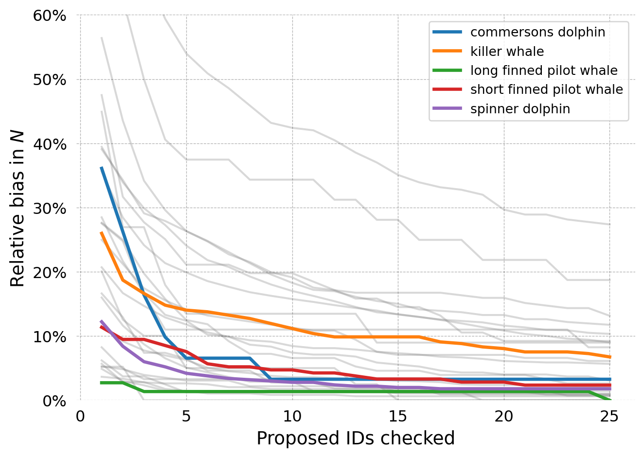
We can translate these false negative rates into expected relative bias in our estimate of the total population size. A relative bias of 10% means that we overestimate the population by 10%. For every one percentage point increase in the false negative rate, our relative bias increases by 2.56 percentage points (Patton et al. 2025). We’re going to exclude the Fraser’s dolphin catalog, which had extremely poor performance.

fn_df = pd.concat(df_list)
fn_df['rbias'] = fn_df['fn_rate'] * 2.56
fn_df = fn_df.loc[fn_df['species'] != 'frasiers_dolphin'].reset_index()

Now we can plot the results for each species. We’ve highlighted five randomly selected species to reduce over plotting.

Code

specials = fn_df.sample(5, random_state=10).species.unique()
special_df = fn_df.loc[fn_df.species.isin(specials)]
nonspecial_df = fn_df.loc[~fn_df.species.isin(specials)]

fig, ax = plt.subplots(figsize = (7, 5), tight_layout=True)

for name, df in nonspecial_df.groupby('species'):
    ax.plot(df.proposed_id_count, df.rbias, alpha=0.3, c='tab:grey', zorder=-2)

for name, df in special_df.groupby('species'):
    ax.plot(df.proposed_id_count, df.rbias, label=name.replace('_', ' '), linewidth=2.5)

import matplotlib.ticker as mtick
ax.yaxis.set_major_formatter(mtick.PercentFormatter(1))

ax.set_ylabel(r'Relative bias in $N$', fontsize=14)
ax.set_xlabel(r'Proposed IDs checked', fontsize=14)
ax.set_ylim((0, 0.6))

ax.spines[:].set_visible(False)

ax.xaxis.tick_bottom()
ax.yaxis.tick_left()

ax.grid(True, 'major', 'both', ls='--', lw=.5, c='k', alpha=.3)

ax.tick_params(axis='both', which='both', labelsize='large',
               bottom=False, top=False, labelbottom=True,
               left=False, right=False, labelleft=True)

ax.legend()

We can see that most species get below 10% once we’ve checked up to 10 proposed matches. In fact, 26 of the 39 datasets achieved a relative bias less than 10% at 10 proposed matches (Patton et al. 2025).

One important caveat that could be depressing performance is that, in this case, we’re matching against all species. As such, the 8th, 9th, 10th, proposed ID for a long-finned pilot whale may indeed by a short-finned pilot whale. In real life, biologists will know not to match against the wrong species. Correcting for this would decrease the false negative rate for all species.

References

Patton, Philip T., Ted Cheeseman, Kenshin Abe, Taiki Yamaguchi, Walter Reade, Ken Southerland, Addison Howard, et al. 2023. “A Deep Learning Approach to Photo–Identification Demonstrates High Performance on Two Dozen Cetacean Species.” Methods in Ecology and Evolution 14 (10): 2611–25.

Patton, Philip T., Krishna Pacifici, Robin W. Baird, Erin M. Oleson, Jason B. Allen, Erin Ashe, Aline Athayde, et al. 2025. “Optimizing Automated Photo Identification for Population Assessments.” Conservation Biology, e14436.