%config InlineBackend.figure_format = 'retina'

from PIL import Image
from pyseter.grade import rate_distinctiveness
from pyseter.sort import load_features
from sklearn.metrics import RocCurveDisplay
import matplotlib.pyplot as plt
import pandas as pd

# load the features
feature_dir = 'working_dir/features'
out_path = feature_dir + '/features.npy'
filenames, feature_array = load_features(out_path)Grading distinctiveness
Pyseter comes with an experimental algorithm for grading individual distinctiveness. This can be useful for partially marked populations, e.g., spinner dolphins.
Background
To understand the distinctiveness algorithm, it can be helpful to first introduce one of Pyseter’s clustering algorithms, NetworkCluster. Network clustering works with similarity scores, which represent the similarity between two individuals in a pair of images. We can define a threshold score, the match_threshold, above which we consider two individuals to be the same. That is, if the similarity score between two images is above a certain threshold, we cluster them into a proposed ID. As such, network clustering works by treating the query set as a network, where the nodes are images and the edges are similarity scores above a threshold. Each set of connected components, i.e., images whose similarity scores are above the match threshold, represents a proposed ID.
We might expect the indistinct individuals to cluster together. In the context of facial recognition, Deng et al. (2023) observed that “unrecognizable identities”, e.g., extremely blurry or masked faces, tend to cluster together. As such, for partially marked populations, the largest cluster in the query set may represent every indistinct individual. Following Deng et al. (2023), we can compute the average feature vector for this cluster. The distance between this average feature vector and the feature vector for each image is the distinctiveness score for that image. As such, the score applies to the image, not the animal. To get a score for an animal, users could average the distinctiveness scores across images for that animal.
Spinner dolphin example
The images in this example were collected during a multi-year photo-ID survey of spinner dolphins in Hawaiʻi. We’ll load in the saved feature vectors from before.
We need to supply two arguments to rate_distinctiveness: the feature_array, and the match_threshold. The lower the match threshold, the more individuals will end up in the unrecognizable identity cluster, potentially including distinct individuals. Conversely, a high match threshold might split the indistinct individuals into many clusters.
distinctiveness = rate_distinctiveness(feature_array, match_threshold=0.5)Unrecognizable identity cluster consists of 196 images./Users/PattonP/miniforge3/envs/pyseter_env/lib/python3.14/site-packages/pyseter/grade.py:35: UserWarning: Distinctiveness grades are experimental and should be verified.
warn(UserWarning('Distinctiveness grades are experimental and should be verified.'))rate_distinctiveness warns you that this is experimental, and lets you know how many individuals ended up in the unrecognizable identity. This should be a quick sanity check.
We can plot the results of the score with the receiver operator characteristic (ROC) curve. This treats the distinctiveness grade as a classifier probability. The area under the curve tells us how good the classifier is, i.e., in terms of the number of false positives and false negatives.
# download the true distinctiveness scores
data_url = (
    'https://raw.githubusercontent.com/philpatton/pyseter/main/'
    'data/spinner-distinct.csv'
)
spinner_distinct = pd.read_csv(data_url)

# merge with the predicted distinctiveness scores
ers_df = pd.DataFrame({'image': filenames, 'ers': distinctiveness})
ers_df = ers_df.merge(spinner_distinct)

# convert distinctiveness to binary outcome such that d1-d2 -> 1
y_score = ers_df['ers']
y_test, _ =  ers_df.distinctiveness.factorize()
y_test = 1 - y_test

fig, ax = plt.subplots(figsize=(5, 4))

ax.hist(y_score[y_test == 1], bins=20, ec='w', alpha=0.7, label='Distinctive')
ax.hist(y_score[y_test == 0], bins=20, ec='w', alpha=0.7, label='Not distinctive')

ax.legend()

ax.spines[['right', 'top']].set_visible(False)

ax.set_xlabel('Embedding recognizability score (ERS)')
ax.set_ylabel('Number of images')

plt.show()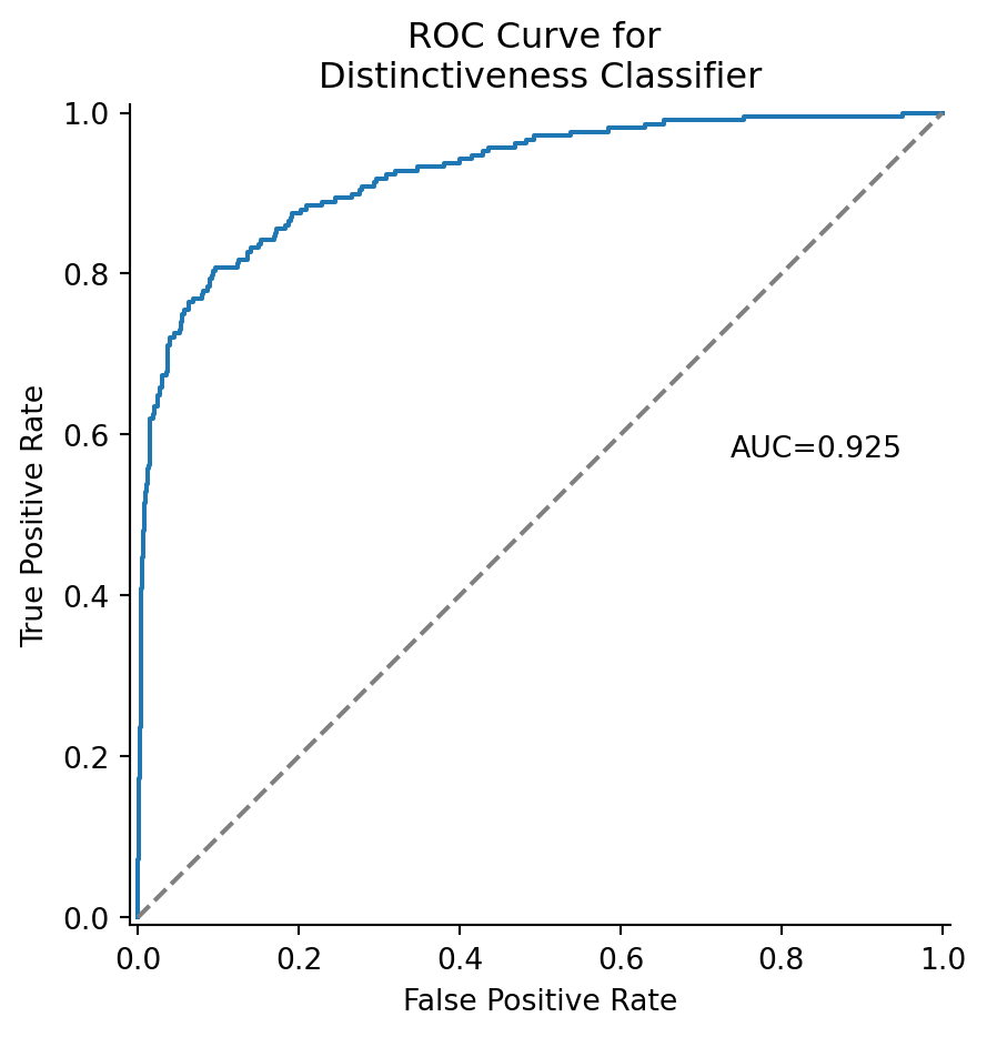
Images of not distinctive individuals (orange bars) rarely have a high ERS. For example, 2.4% of indistinct individuals and 42% of distinct individuals have an ERS greater than 0.8. We can look at the outlier images of indistinct individuals with a high ERS.
outliers = ers_df.loc[(ers_df.distinctiveness == 'd3-d4') & (ers_df.ers > 0.8), 'image']
fig, axes = plt.subplots(3, 2, figsize=(8, 9))

for i, image in enumerate(outliers):
    ax = axes.flat[i]
    path = 'working_dir/all_images/' + image
    img = Image.open(path)
    ax.imshow(img)
    ax.axis('off')

axes[2, 1].remove()
fig.suptitle('Indistinct individuals ERS > 0.8')

plt.tight_layout()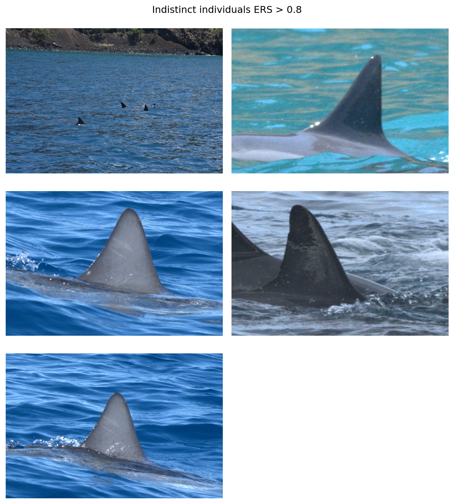
One of the images (top left) is clearly a cropping error. Two of the images depict an individual with some rake marks across the dorsal fin that AnyDorsal might be keying in on. The individual in the middle right does have some notches along its fin. It’s unclear what AnyDorsal sees in the image in the upper right hand corner
Additionally, we can see that distinctive individuals (blue) rarely have a low ERS Figure 1. While 0.57% of distinct individuals and have an ERS less than 0.5, that number is 43% for indistinct individuals. We can look at the six outlier distinctive individuals with an ERS below 0.5.
outliers = ers_df.loc[(ers_df.distinctiveness == 'd1-d2') & (ers_df.ers < 0.5), 'image']
fig, axes = plt.subplots(3, 2, figsize=(8, 9))

for i, image in enumerate(outliers):
    ax = axes.flat[i]
    path = 'working_dir/all_images/' + image
    img = Image.open(path)
    ax.imshow(img)
    ax.axis('off')

fig.suptitle('Distinctive individuals with ERS < 0.5')

plt.tight_layout()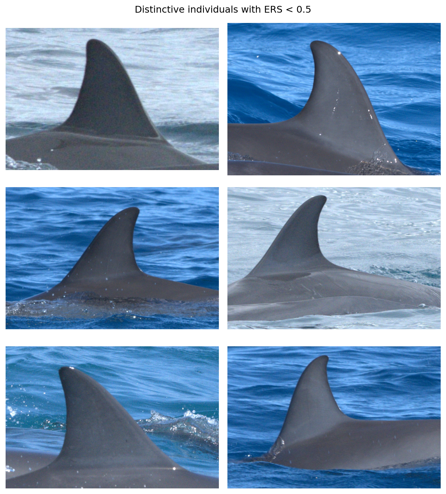
The images show relatively clean fins but with certain characteristics (e.g., fin shape), that stood out to human reviewers as distinctive enough for classification.
Another way to assess the usefulness of the ERS is to treat it as a classifier where \(I(\mathrm{ers} > \tau) = 1\) for some threshold \(\tau\). We can evaluate the classifier with an ROC curve.
display = RocCurveDisplay.from_predictions(
    y_test, y_score, name="ERS", plot_chance_level=True, despine=True
)

fig = display.figure_
fig.set_size_inches(5, 5)
ax = display.ax_.axes
ax.set_title('ROC curve for ERS classifier of distinctiveness')
ax.set_ylabel('True positive rate (Positive label: Distinctive)')
ax.set_xlabel('False positive rate (Positive label: Distinctive)')

plt.show()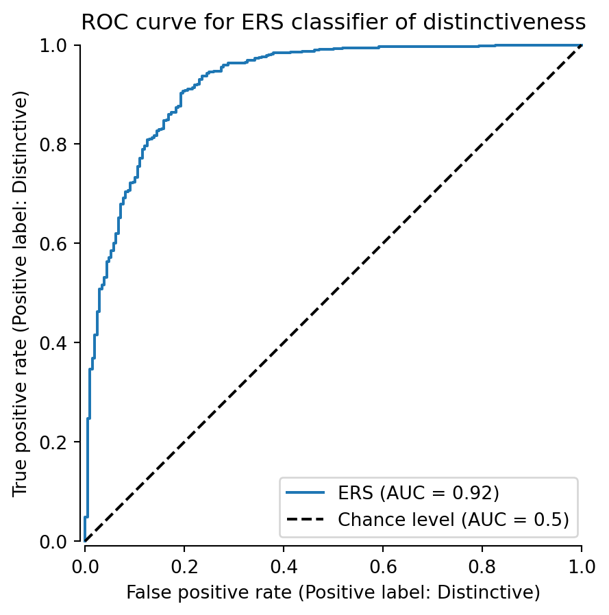
We can see that the classifier achieves an AUC of 0.92, outperforming the random classifier (AUC = 0.5). The true positive rate grow rapidly initially because there are so few distinct individuals with low ERS Figure 1. Then, the curve begins to sag a bit as it enters the area of overlap between 0.4 and 0.6 ERS Figure 1.
We can also try to visualize the feature vectors with UMAP (McInnes et al. 2018). Interpreting UMAP is a minefield of caveats, but it can be a useful visualization technique for extremely high dimensional spaces. The feature vectors reside on a 5,504 dimensional hypersphere.
import umap

# project the embeddings with UMAP
embedding = umap.UMAP(
    min_dist = 0.55, n_neighbors=25, metric='cosine'
).fit_transform(feature_array)


fig, ax = plt.subplots(figsize=(5, 5), tight_layout=True)

indistinct = embedding[y_test == 0]
ax.scatter(indistinct[:, 0], indistinct[:, 1], s=5, label='Not Distinctive',
           color='C1', zorder=2)

distinct = embedding[y_test == 1]
ax.scatter(distinct[:, 0], distinct[:, 1], s=5, label='Distinctive', color='C0',
           zorder=-2, alpha=0.8)

ax.set_xticks([])
ax.set_yticks([])
ax.legend()

ax.set_title(f'UMAP projection of feature vectors')

plt.show()
UMAP echoes our previous results, namely, that the embeddings for the not distinctive individuals tend to cluster together. There is, however, substantial overlap, and there are a few not distinctive embeddings lingering where they shouldn’t (at least theoretically).
Warning
Users will need to install umap-learn, e.g., conda install umap-learn -c conda-forge, to run the above code block
References
Deng, Siqi, Yuanjun Xiong, Meng Wang, Wei Xia, and Stefano Soatto. 2023. “Harnessing Unrecognizable Faces for Improving Face Recognition.” In Proceedings of the IEEE/CVF Winter Conference on Applications of Computer Vision, 3424–33.
McInnes, Leland, John Healy, Nathaniel Saul, and Lukas Großberger. 2018. “UMAP: Uniform Manifold Approximation and Projection.” Journal of Open Source Software 3 (29): 861. https://doi.org/10.21105/joss.00861.