%config InlineBackend.figure_format = 'retina'

from pyseter.sort import load_features
from pyseter.identify import predict_ids
import matplotlib.pyplot as plt
import pandas as pd

# load in the feature vectors
data_dir = '/Users/PattonP/datasets/happywhale/'
feature_dir = data_dir + '/features'

reference_path = feature_dir + '/train_features.npy'
reference_files, reference_features = load_features(reference_path)

query_path = feature_dir + '/test_features.npy'
query_files, query_features = load_features(query_path)Evaluating AnyDorsal
In this notebook, we’ll demonstrate how do evaluate AnyDorsal’s’ performance on a test dataset. We’ll use the Happy Whale and Dolphin Kaggle competition dataset as an example. You can download the data by following that linked page (click the big “Download all” button). FYI, you’ll have to create an account first.
In the Predicting IDs notebook, we demonstrated how to extract features for the Happywhale dataset using a set of bounding boxes. Here, we’ll load the features in.
In order to evaluate the performance of AnyDorsal on the test set, we’ll need to know the IDs of animals in the train set and the test set.
data_url = (
    'https://raw.githubusercontent.com/philpatton/pyseter/main/'
    'data/happywhale-ids.csv'
)
id_df = pd.read_csv(data_url)

# fix known species errors
id_df.replace(
    {
        "globis": "short_finned_pilot_whale",
        "pilot_whale": "short_finned_pilot_whale",
        "kiler_whale": "killer_whale",
        "bottlenose_dolpin": "bottlenose_dolphin"
    },
    inplace=True
)

id_df.head(10)| image | species | individual_id | |
|---|---|---|---|
| 0 | 000110707af0ba.jpg | gray_whale | fbe2b15b5481 |
| 1 | 00021adfb725ed.jpg | melon_headed_whale | cadddb1636b9 |
| 2 | 000562241d384d.jpg | humpback_whale | 1a71fbb72250 |
| 3 | 0006287ec424cb.jpg | false_killer_whale | 1424c7fec826 |
| 4 | 0007c33415ce37.jpg | false_killer_whale | 60008f293a2b |
| 5 | 0007d9bca26a99.jpg | bottlenose_dolphin | 4b00fe572063 |
| 6 | 000809ecb2ccad.jpg | beluga | 1ce3ba6a3c29 |
| 7 | 00087baf5cef7a.jpg | humpback_whale | 8e5253662392 |
| 8 | 00098d1376dab2.jpg | humpback_whale | c4274d90be60 |
| 9 | 000a8f2d5c316a.jpg | bottlenose_dolphin | b9907151f66e |
Code
# excel on mac corrupts the IDs (no need to do this on PC or linux)
id_df['individual_id'] = id_df['individual_id'].apply(
    lambda x: str(int(float(x))) if 'E+' in str(x) else x
)
Now we’ll predict the IDs in the query set.
query_dict = dict(zip(query_files, query_features))
reference_dict = dict(zip(reference_files, reference_features))

prediction_df = predict_ids(reference_dict, query_dict, id_df, proposed_id_count=5)
prediction_df.head(20)| image | rank | predicted_id | score | |
|---|---|---|---|---|
| 0 | a704da09e32dc3.jpg | 1 | 5f2296c18e26 | 0.500233 |
| 1 | a704da09e32dc3.jpg | 2 | new_individual | 0.500000 |
| 2 | a704da09e32dc3.jpg | 3 | 61f9e4cd30eb | 0.432061 |
| 3 | a704da09e32dc3.jpg | 4 | cb372e9b2c48 | 0.411830 |
| 4 | a704da09e32dc3.jpg | 5 | 43dad7ffa3c7 | 0.405389 |
| 5 | de1569496d42f4.jpg | 1 | ed237f7c2165 | 0.826259 |
| 6 | de1569496d42f4.jpg | 2 | new_individual | 0.500000 |
| 7 | de1569496d42f4.jpg | 3 | 8c4a71fd3eb1 | 0.446297 |
| 8 | de1569496d42f4.jpg | 4 | 7d4deec3b721 | 0.424570 |
| 9 | de1569496d42f4.jpg | 5 | fcc7ade0c50a | 0.376511 |
| 10 | 4ab51dd663dd29.jpg | 1 | b9b24be2d5ae | 0.680653 |
| 11 | 4ab51dd663dd29.jpg | 2 | 31f748b822f4 | 0.503390 |
| 12 | 4ab51dd663dd29.jpg | 3 | new_individual | 0.500000 |
| 13 | 4ab51dd663dd29.jpg | 4 | 7845337998d6 | 0.497671 |
| 14 | 4ab51dd663dd29.jpg | 5 | efda8f368763 | 0.455688 |
| 15 | da27c3f9f96504.jpg | 1 | c02b7ad6faa0 | 0.937102 |
| 16 | da27c3f9f96504.jpg | 2 | new_individual | 0.500000 |
| 17 | da27c3f9f96504.jpg | 3 | 70858f1edf62 | 0.375488 |
| 18 | da27c3f9f96504.jpg | 4 | 72b0033dd4fd | 0.367204 |
| 19 | da27c3f9f96504.jpg | 5 | 749e56a8ec71 | 0.354002 |
Top 5%
We can evaluate the performance with several metrics, including Top 5%, or top 5 accuracy, which is just the percentage of times that the correct answer was one of the top five predictions. To do so, we need to compute the rank of the prediction, that is, the location of the correct ID in the proposed IDs for every image in the test set.
One way to do so is to merge the ID DataFrame with the prediction DataFrame, using both image and ID columns as keys. We’ll do a left join, such that when the true ID is one of the proposed IDs, the prediction, its rank and score are returned. When true true ID is not one of the proposed IDs, we’ll get NAs for those columns. We can check to see that it worked by checking the number of rows in the result (there are 27956 images in the testing dataset).
# add the predictions and the scores to the id dataframe
performance_df = id_df.merge(
    prediction_df,
    how='left',
    left_on=['image', 'individual_id'],
    right_on=['image', 'predicted_id']
)

# filter out the training images
train_images = pd.read_csv(data_dir + '/train.csv').image
performance_df = performance_df.loc[~performance_df.image.isin(train_images)]
print(performance_df.shape)
(27956, 6)performance_df.head(20)| image | species | individual_id | rank | predicted_id | score | |
|---|---|---|---|---|---|---|
| 0 | 000110707af0ba.jpg | gray_whale | fbe2b15b5481 | 1.0 | fbe2b15b5481 | 0.871143 |
| 3 | 0006287ec424cb.jpg | false_killer_whale | 1424c7fec826 | 1.0 | 1424c7fec826 | 0.794225 |
| 6 | 000809ecb2ccad.jpg | beluga | 1ce3ba6a3c29 | 1.0 | 1ce3ba6a3c29 | 0.797251 |
| 8 | 00098d1376dab2.jpg | humpback_whale | c4274d90be60 | 1.0 | c4274d90be60 | 0.816240 |
| 10 | 000b8d89c738bd.jpg | dusky_dolphin | new_individual | 1.0 | new_individual | 0.500000 |
| 15 | 000e246888710c.jpg | melon_headed_whale | new_individual | 2.0 | new_individual | 0.500000 |
| 16 | 000eb6e73a31a5.jpg | bottlenose_dolphin | 77410a623426 | 1.0 | 77410a623426 | 0.709175 |
| 17 | 000fe6ebfc9893.jpg | spinner_dolphin | 8805324885f2 | 1.0 | 8805324885f2 | 0.942707 |
| 20 | 0011f7a65044e4.jpg | spinner_dolphin | d5dcbb35777c | 1.0 | d5dcbb35777c | 0.676094 |
| 21 | 0012ff300032e3.jpg | beluga | 19b638e11443 | 1.0 | 19b638e11443 | 0.950292 |
| 23 | 00150406ce5395.jpg | false_killer_whale | 2280b5fcc6c2 | 1.0 | 2280b5fcc6c2 | 0.837772 |
| 25 | 0016cd18d6410e.jpg | cuviers_beaked_whale | 65620eadc0b4 | 1.0 | 65620eadc0b4 | 0.582929 |
| 27 | 0017a9c11c61a8.jpg | beluga | new_individual | 2.0 | new_individual | 0.500000 |
| 29 | 0017f7e0de07b1.jpg | bottlenose_dolphin | 81bec36eb86e | 1.0 | 81bec36eb86e | 0.840179 |
| 32 | 001c4c6d532419.jpg | bottlenose_dolphin | 2efee119d786 | 1.0 | 2efee119d786 | 0.748652 |
| 34 | 001dc45839b1b5.jpg | southern_right_whale | cd2e1d83c6a1 | 1.0 | cd2e1d83c6a1 | 0.791898 |
| 35 | 001ea84d905ced.jpg | humpback_whale | 02f5c5ee9c2a | 1.0 | 02f5c5ee9c2a | 0.680320 |
| 43 | 00248b9385e2e0.jpg | blue_whale | 67b7b6934db9 | 1.0 | 67b7b6934db9 | 0.509903 |
| 48 | 002c7034834e2c.jpg | killer_whale | ed15fd01efbe | 1.0 | ed15fd01efbe | 0.815825 |
| 49 | 002d7a5f6d6765.jpg | beluga | 3a055fad1478 | NaN | NaN | NaN |
Any image with an NA rank means that the true ID was not one of the proposed_ids. We’ll fill those with some large value, say, 9999. Then, we just need to compute the average number of times that the rank was less than 6.
performance_df['rank'] = performance_df['rank'].fillna(9999)
performance_df['in_top_5'] = performance_df['rank'] < 6
print(f'Top 5%: {performance_df.in_top_5.mean():0.1%}')
Top 5%: 92.1%We can see that the correct answer was in the top 5 predictions for 92% of test images. For fun, we can look at this performance across species.
import matplotlib.pyplot as plt
import matplotlib.ticker as mtick

plt.style.use('fivethirtyeight')
plt.rcParams['axes.facecolor'] = 'white'
plt.rcParams['figure.facecolor'] = 'white'

map_df = (
    performance_df.groupby('species')
        .in_top_5
        .mean()
        .rename('top5')
        .reset_index()
        .sort_values('top5')
)
map_df.species = map_df.species.str.replace('_', ' ')

fig, ax = plt.subplots(figsize=(4, 8))
ax.scatter(map_df.top5, map_df.species)
for row in map_df.itertuples():
    ax.text(row.top5 - 0.02, row.species, f'{row.top5:0.0%}', ha='right',
            va='center', fontsize=12)
ax.xaxis.set_major_formatter(mtick.PercentFormatter(1))
ax.set_title('AnyDorsal Performance')
ax.set_xlabel('Top 5%')
ax.set_xlim((0,1.03))
plt.show()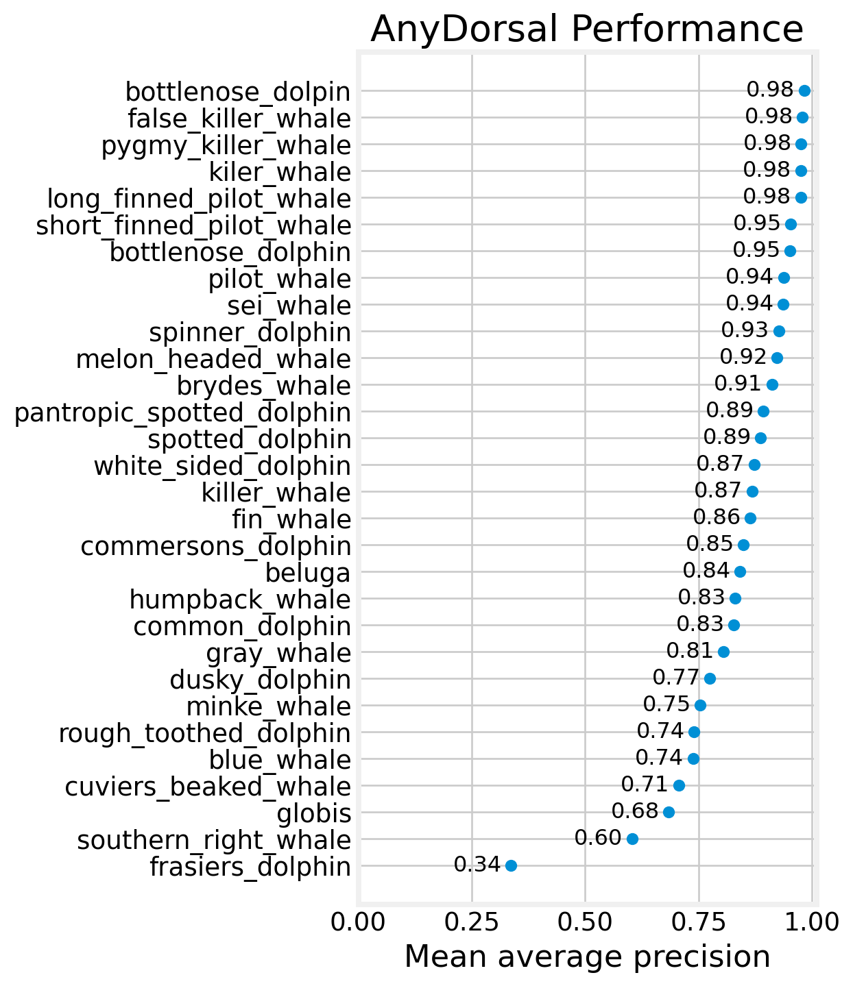
We can see that the 12 of 24 species achieve a Top 5% of over 95%. Some of these species are being rewarded (or punished) by the prevalence of new_individuals in the dataset, since new_individual is almost always one of the top 5 proposed IDs.
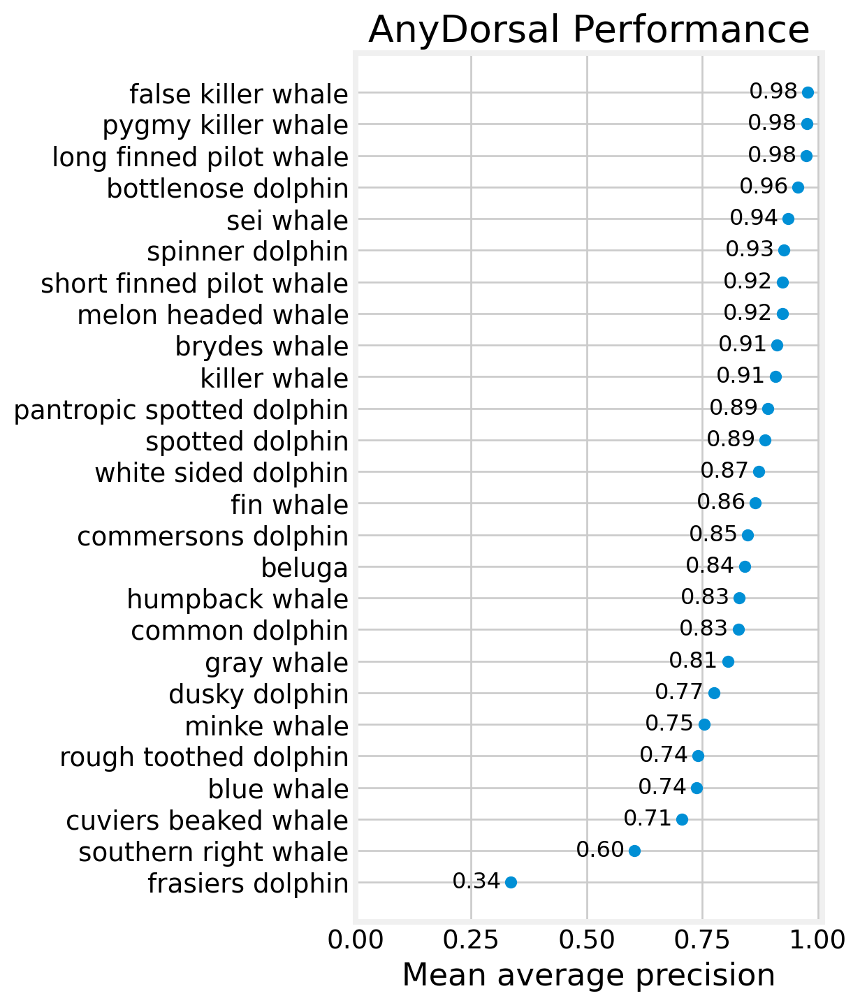
Mean average precision
We can also evaluate AnyDorsal with Mean Average Precision (MAP), a slightly more rigorous metric. MAP evaluates a set of predictions, in this case, a set of 5 predictions. For a set of five ordered predictions, the precision score will be \(1/1 = 1\) if the first prediction is correct, \(1/2\) if the second is correct, and so on until \(1/5\) if the fifth prediction is correct, or \(0\) if none of the five predictions are correct. As such, the precision is just the reciprocal of the rank. Recall that we set the NA values to 9999 earlier, and \(1/9999 \approx 0\). MAP is the mean precision score for a set.
performance_df['precision'] = 1 / performance_df['rank']
map5 = performance_df.precision.mean()
print(f'MAP@5: {map5:0.3f}')
MAP@5: 0.863For fun, we can look at the results by species
map_df = (
    performance_df.groupby('species')
        .precision
        .mean()
        .rename('MAP')
        .reset_index()
        .sort_values('MAP')
)
map_df.species = map_df.species.str.replace('_', ' ')

fig, ax = plt.subplots(figsize=(4, 8))
ax.scatter(map_df.MAP, map_df.species)
for row in map_df.itertuples():
    ax.text(row.MAP - 0.02, row.species, f'{row.MAP:0.2f}', ha='right',
            va='center', fontsize=12)
ax.set_xlim((0,1.01))
ax.set_title('AnyDorsal Performance')
ax.set_xlabel('Mean average precision')
plt.show()