In this notebook, I explore fitting community occupancy models in PyMC. Community occupancy models are a multi-species extension of standard occupancy models. The benefit of these models is that, by treating each species as a random effect, they can estimate occupancy and detection more precisely than single species models. Further, through data augmentation, they can estimate the richness of the supercommunity, that is, the total number of species that use the study area during the surveys.
US Breeding Bird Survey
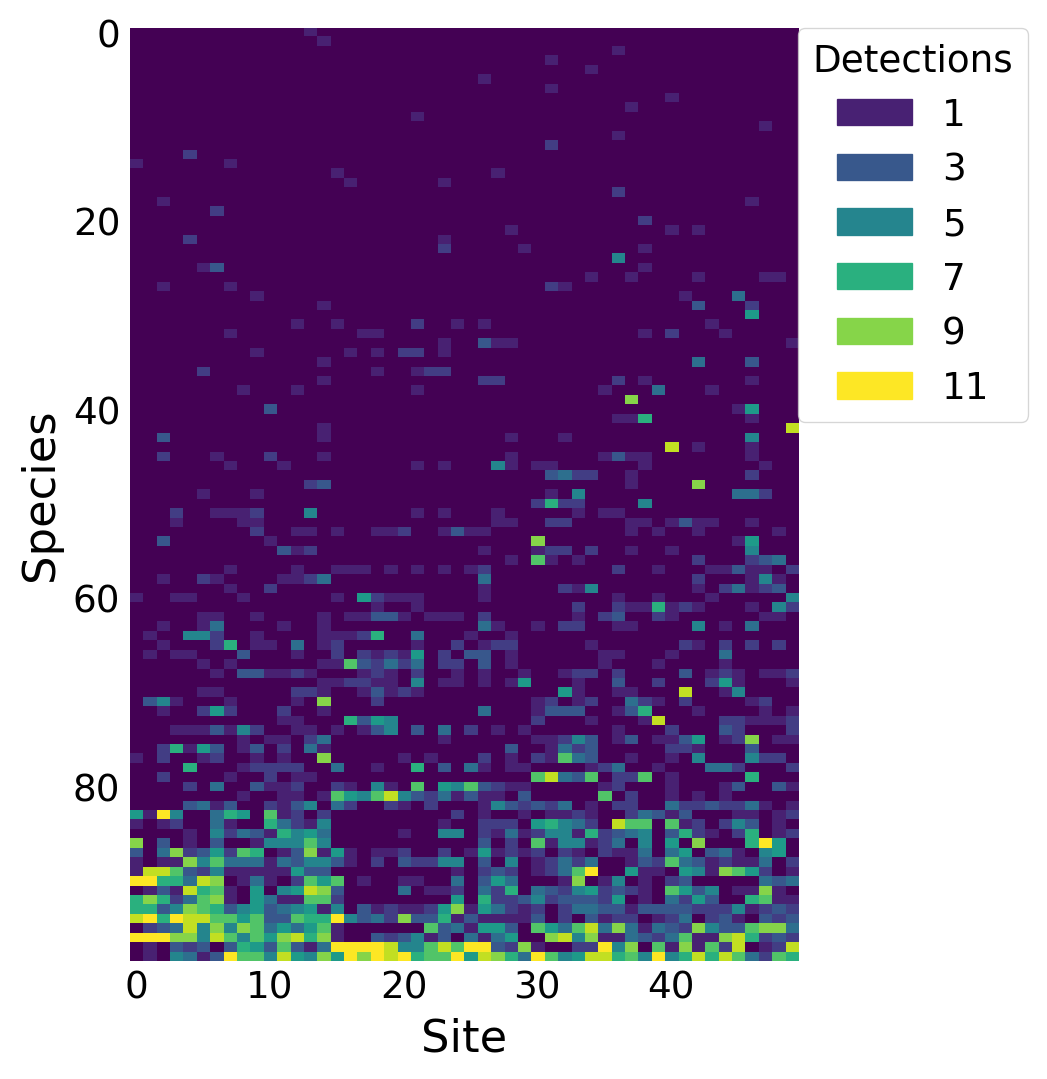
As a motivating example, I use the breeding bird survey (BBS) data used by Dorazio and Royle (2005) and Royle and Dorazio (2008), Chapter 12. This is a \((n, J)\) matrix with the number of times each species was detected over \(K\) surveys, where \(n\) is the number of detected species and \(J\) is the number surveyed sites. In this example, \(n=99\) species were detected at the \(J=50\) sites over the \(K=11\) surveys in New Hampshire. The BBS occurs on routes across the US. This dataset represents one route.
%config InlineBackend.figure_format ='retina'from matplotlib.patches import Patchfrom scipy.stats import binomimport arviz as azimport matplotlib.pyplot as pltimport numpy as npimport pandas as pdimport pymc as pmimport seaborn as sns# only necessary on MacOS Sequoia# https://discourse.pymc.io/t/pytensor-fails-to-compile-model-after-upgrading-to-mac-os-15-4/16796/5import pytensorpytensor.config.cxx ='/usr/bin/clang++'SEED =808RNG = np.random.default_rng(SEED)plt.style.use('fivethirtyeight')plt.rcParams['axes.facecolor'] ='white'plt.rcParams['figure.facecolor'] ='white'plt.rcParams['axes.spines.left'] =Falseplt.rcParams['axes.spines.right'] =Falseplt.rcParams['axes.spines.top'] =Falseplt.rcParams['axes.spines.bottom'] =Falsesns.set_palette("tab10")def invlogit(x):return1/ (1+ np.exp(-x))# read in the detection datanh17 = pd.read_csv('detectionFreq.NH17.csv')Y = nh17.to_numpy()n, J = Y.shapeK = Y.max()# convert the species names to intsspecies_idx, lookup = nh17.index.factorize() # lookup[int] returns the actual name# plot the detection frequenciesfig, ax = plt.subplots(figsize=(4, 6))im = ax.imshow(Y[np.argsort(Y.sum(axis=1))], aspect='auto')ax.set_ylabel('Species')ax.set_xlabel('Site')# add a legendvalues = np.unique(Y.ravel())[1::2]colors = [ im.cmap(im.norm(value)) for value in values]patches = [ Patch(color=colors[i], label=f'{v}') for i, v inenumerate(values) ]plt.legend(title='Detections', handles=patches, bbox_to_anchor=(1, 1), loc=2, borderaxespad=0.)ax.grid(False)plt.show()
Figure 1: Number of detections for each species at each site along this BBS route.
Dorazio and Royle (2005) draw each species-level effect from a multivariate normal distribution, \[
{\alpha_i \choose \beta_i} \sim \text{Normal} \left( {\mu_{\,\text{detection}} \choose \mu_{\, \text{occupancy}}}, \; \mathbf{\Sigma} \right),
\] where \(\alpha_i\) is the logit-scale probability of detection for species \(i=1,\dots,n\), \(\beta_i\) is the logit-scale probability of occurrence, \(\mu\) is the community-level average, and \(\mathbf{\Sigma}\) is the covariance matrix. We assume that there will be a positive correlation between occupancy and the probability of detection, since abundance is positively correlated with both.
Known \(N\)
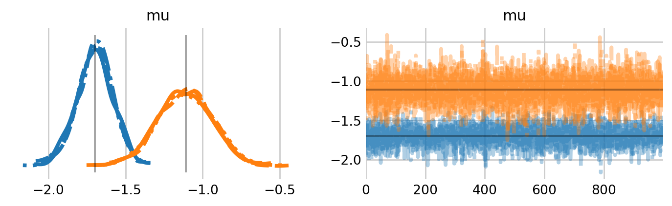
First, I fit the the known \(N\) version of the model. The goal of this version is to estimate occurrence and detection for each species, without estimating species richness.
This notebook makes extensive use of the coords feature in PyMC. Coords makes it easier to incorporate the species-level effects via the multivariate normal. I use a \(\text{Normal}(0, 2)\) prior for both \(\mu\) parameters, and a LKJ Cholesky covariance prior for \(\mathbf{\Sigma}.\)
Throughout the notebook, I use the nutpie sampler within PyMC. Nutpie is a NUTS sampler written in Rust, and is often faster than PyMC.
coords = {'process': ['detection', 'occurrence'],'process_bis': ['detection', 'occurrence'],'species': lookup}with pm.Model(coords=coords) as known:# priors for community-level means for detection and occurrence mu = pm.Normal('mu', 0, 2, dims='process')# prior for covariance matrix for occurrence and detection chol, corr, stds = pm.LKJCholeskyCov("chol", n=2, eta=2.0, sd_dist=pm.Exponential.dist(1.0, shape=2) ) cov = pm.Deterministic("cov", chol.dot(chol.T), dims=("process", "process_bis"))# species-level occurrence and detection probabilities on logit-scale ab = pm.MvNormal("ab", mu, chol=chol, dims=("species", "process"))# probability of detection. newaxis allows for broadcasting a = ab[:, 0][:, np.newaxis] p = pm.Deterministic("p", pm.math.invlogit(a))# probability of detection. newaxis allows for broadcasting b = ab[:, 1][:, np.newaxis] psi = pm.Deterministic("psi", pm.math.invlogit(b))# likelihood pm.ZeroInflatedBinomial('Y', p=p, psi=psi, n=K, observed=Y)pm.model_to_graphviz(known)
Figure 2: Visual representation of the known \(N\) version of the community occupancy model.
with known:
    known_idata = pm.sample(nuts_sampler='nutpie')
Figure 3: Trace plots for the community level means of occupancy and abundance in the known \(N\) version of the BBS model. The estimates from Royle and Dorazio (2008) are shown by vertical and horizontal lines.
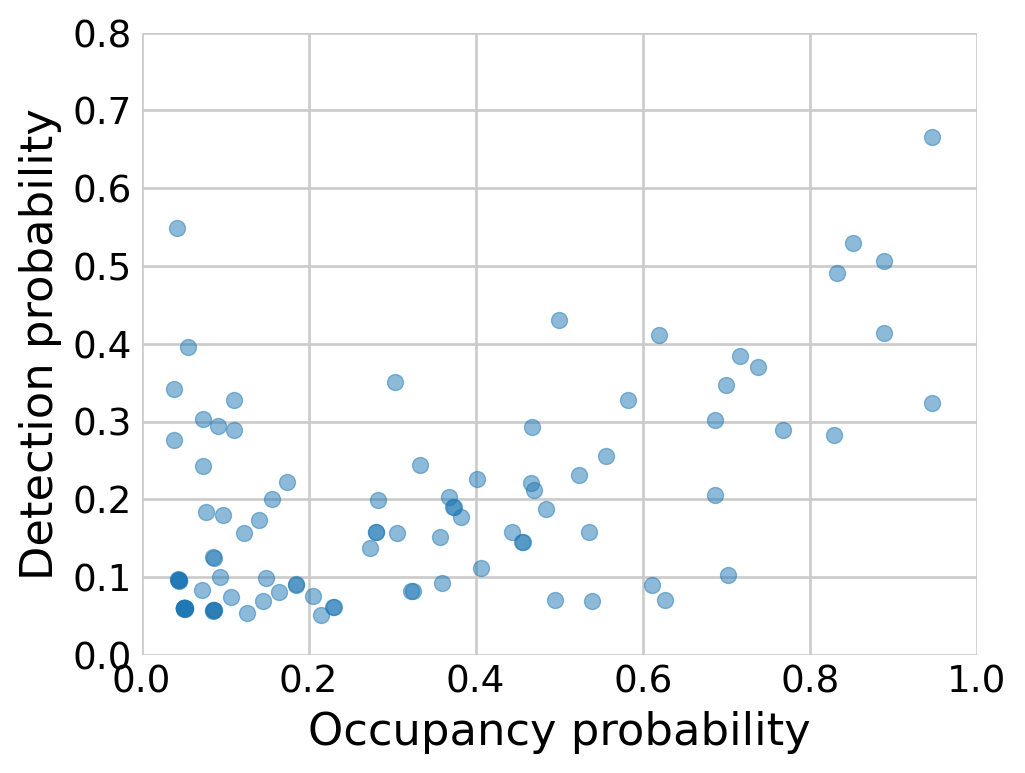
Figure 4: Species-level probabilities of detection and occupancy.
The estimates of the community-level means is quite close to the estimates from Royle and Dorazio (2008). We can visualize the species-level probabilities of detection and occupancy. Compare with Figure 12.3 in Royle and Dorazio (2008).
Unknown \(N\)
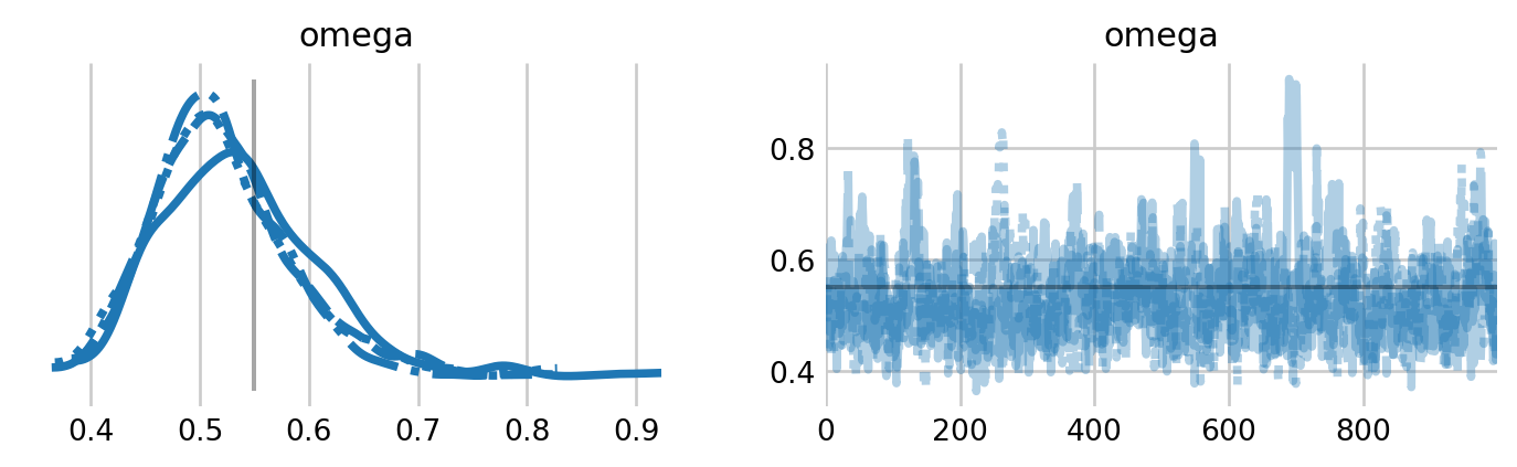
Next, I train the unknown \(N\) version of the model. Like many other notebooks in this series, it relies on augmenting the detection histories with all-zero histories. These represent the detection histories for species that may use the study site, but were not detected over the \(K=11\) surveys. I also augment the species names in the coords dict, such that we can still use the dims argument in the multivariate normal. Mirroring Royle and Dorazio (2008), I augment the history \(M - n\) all-zero histories, where \(M=250\) and \(n\) is the number of species detected during the survey.
The CustomDist class
In the notebooks for closed models, we have relied on the marginalize function from pymc_extras. In my testing, however, this function fails with this model, perhaps because of the the double layers of zero inflation (site occupation, community inclusion). As such, we will have to marginalize the discrete latent state ourselves. To do so, we have to create a custom distribution via PyMC’s CustomDist class. The typical way to do so is to define the logp as a function, as one would in Stan.
M =250all_zero_history = np.zeros((M - n, J))Y_augmented = np.row_stack((Y, all_zero_history))aug_names = [f'aug{i}'for i in np.arange(M - n)]spp_aug = np.concatenate((lookup, aug_names))coords = {'process': ['detection', 'occurrence'],'process_bis': ['detection', 'occurrence'],'species_aug': spp_aug}def logp(x, psi, n, p, omega): rv = pm.ZeroInflatedBinomial.dist(psi=psi, n=n, p=p) lp = pm.logp(rv, x) lp_sum = lp.sum(axis=1) lp_exp = pm.math.exp(lp_sum) res = pm.math.switch( x.sum(axis=1) >0, lp_exp * omega, lp_exp * omega + (1- omega) )return pm.math.log(res)with pm.Model(coords=coords) as unknown:# priors for inclusion omega = pm.Beta('omega', 0.001, 1)# priors for community-level means for detection and occurrence mu = pm.Normal('mu', 0, 2, dims='process')# prior for covariance matrix for occurrence and detection chol, corr, stds = pm.LKJCholeskyCov("chol", n=2, eta=2.0, sd_dist=pm.Exponential.dist(1.0, shape=2) ) cov = pm.Deterministic("cov", chol.dot(chol.T), dims=("process", "process_bis"))# species-level occurrence and detection probabilities on logit-scale ab = pm.MvNormal("ab", mu, chol=chol, dims=("species_aug", "process"))# probability of detection alpha = ab[:, 0] p = pm.Deterministic("p", pm.math.invlogit(alpha))# probability of occurrence beta = ab[:, 1] psi = pm.Deterministic("psi", pm.math.invlogit(beta))# likelihood pm.CustomDist('Y', psi[:, np.newaxis], K, p[:, np.newaxis], omega, logp=logp, observed=Y_augmented )pm.model_to_graphviz(unknown)
/var/folders/7b/nb0vyhy90mdf30_65xwqzl300000gn/T/ipykernel_47331/4077413751.py:3: DeprecationWarning: `row_stack` alias is deprecated. Use `np.vstack` directly.
  Y_augmented = np.row_stack((Y, all_zero_history))
Figure 5: Visual representation of the unknown \(N\) version of the BBS model.
with unknown: unknown_idata = pm.sample(nuts_sampler='nutpie')# unknown_idata = pm.sample()
Sampler Progress
Total Chains: 4
Active Chains: 0
Finished Chains:
4
Sampling for 24 seconds
Estimated Time to Completion:
now
Progress
Draws
Divergences
Step Size
Gradients/Draw
2000
0
0.27
15
2000
0
0.27
15
2000
0
0.26
15
2000
0
0.26
15
We see some warnings about the effective sample size and the \(\hat{R}\) statistic. Some of these warnings may just relate to the individual random effects.
Figure 6: Trace plots for the inclusion parameter for the unknown \(N\) version of the BBS model. The estimate from Royle and Dorazio (2008) are shown by vertical and horizontal lines.
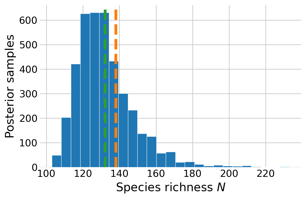
I can plot the posterior distribution of species richness \(N.\) This is slightly more complicated than before sinc there is an additional level of zero-inflation (included and never detected or not-included) in this model compared to the occupancy model (present and never detection or not present).
# relevant posterior samplespost = az.extract(unknown_idata)o_samps = post.omega.to_numpy()# only care about the undetected speciesp_samps = post.p.to_numpy()[n:]# probability that the species was in the study area but wasn't detectedp_if_present = o_samps * binom.pmf(0, n=K, p=p_samps)p_total = p_if_present + (1- o_samps)# simulate the latent occurrence state for the undetected speciesZ = RNG.binomial(1, p_if_present / p_total)# simulate species richnessnumber_undetected = Z.sum(axis=0)N_samps = number_undetected + n# relevant posterior samples# post = az.extract(unknown_idata)# o_samps = post.omega.to_numpy()# N_samps = RNG.binomial(M, o_samps)# posterior distributionN_hat_royle =138fig, ax = plt.subplots(figsize=(6, 4))ax.hist(N_samps, edgecolor='white', bins=25)ax.set_xlabel('Species richness $N$')ax.set_ylabel('Posterior samples')ax.axvline(N_hat_royle, linestyle='--', color='C1')ax.axvline(N_samps.mean(), linestyle='--', color='C2')plt.show()
Figure 7: Posterior distribution of species richness from the BBS model.
%load_ext watermark%watermark -n -u -v -iv -w
Last updated: Tue Oct 14 2025

Python implementation: CPython
Python version       : 3.13.2
IPython version      : 9.0.2

numpy     : 2.1.3
pymc      : 5.22.0
pytensor  : 2.30.2
matplotlib: 3.10.1
pandas    : 2.2.3
arviz     : 0.21.0
seaborn   : 0.13.2

Watermark: 2.5.0
References
Dorazio, Robert M, and J Andrew Royle. 2005. “Estimating Size and Composition of Biological Communities by Modeling the Occurrence of Species.”Journal of the American Statistical Association 100 (470): 389–98.
Royle, J Andrew, and Robert M Dorazio. 2008. Hierarchical Modeling and Inference in Ecology: The Analysis of Data from Populations, Metapopulations and Communities. Elsevier.